1. scVMAP process
scVMAP: https://bio.liclab.net/scvmap/scVMAP reproducibility: https://github.com/YuZhengM/scvmap_reproducibilityscVMAP tutorial: https://scvmap.readthedocs.io/en/latest/scVMAP front-end: https://github.com/YuZhengM/scvmap_webscVMAP back-end: https://github.com/YuZhengM/scvmap
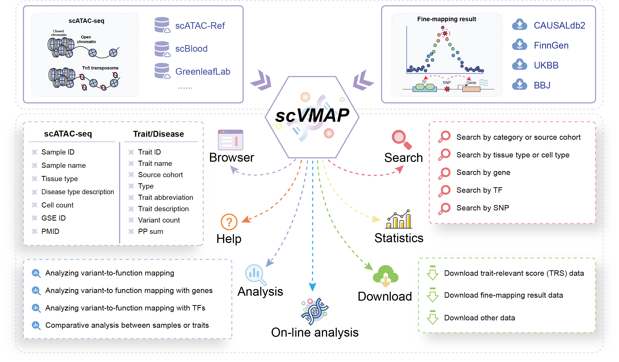
scVMAP gathers and provides scATAC-seq datasets with established cell type labels (from scATAC-Ref, GreenleafLab and PlaqView) and cell type labels annotated by singleR (from scBlood), along with detailed fine-mapping data (from CAUSALdb2, FinnGen, UKBB and BBJ). scVMAP, by employing the SCAVENGE and g-chromVAR methods, assigns trait-relevant scores at single-cell resolution, uncovering biologically relevant cell types.
The core original intention and purpose of scVMAP is to provide a resource of trait-relevant significant cell types, offering researchers interested in this objective a convenient and fast retrieval interface. It uses widely recognized methods to provide reference for key variants, TFs, and genes involved in relevant potential enrichment mechanisms, offering researchers a direction for reference, reducing their time, and making a modest contribution to the scientific research community.
Throughout the process, data undergoes standardization, unified processing, and comprehensive analysis. The main contents are as follows:
Single-cell samples:
Differential gene activity analysis of cell types
Differential TF activity analysis of cell types
High-scoring gene pathway enrichment analysis of cell types
Traits or diseases:
LD-based MAGMA analysis (Trait-relevant genes)
HOMER motif enrichment analysis (Trait-relevant TFs)
MAGMA-based trait-relevant gene pathway enrichment analysis
Integrated analysis:
ATAC-based Cicero analysis (Trait-relevant genes)
ATAC-based GimmeMotifs analysis (Trait-relevant genes)
Gene hub regulatory network analysis
TF hub regulatory network analysis
Integrated regulatory network analysis
The scVMAP database primarily provides the following functions: Data-browse, Search, Analysis, Statistics, Download, Contact, and Online analysis.
These functionalities streamline the process of studying single-cell genetic regulation, enabling users to easily explore and interpret biological mechanisms in specific contexts.
In conclusion, (scVMAP, https://bio.liclab.net/scvmap/) is a user-centric database that facilitates the exploration and interpretation of single-cell genetic data through structured displays and dynamic visualizations. It offers intuitive workflows, customizable parameters and comprehensive data accessibility.
Tip
This section provides a comprehensive explanation of the entire pipeline for the scVMAP platform, encompassing the stages of data acquisition, curation, analysis, and the ultimate platform realization.
1.1 Data processing methods
We provide the software and version information required for data processing in the scVMAP platform, along with the corresponding code to reproduce the results.
1.2 Data collection and curation
The scVMAP platform collects scATAC-seq data and fine-mapping result data.
1.2.1 Collection of scATAC-seq data
The collected scATAC-seq data mainly comes from scATAC-Ref, scBlood, GreenleafLab, and PlaqView sources.
A total of 183 single-cell sample data were collected, with detailed information as follows:
Download url: sample_info_with_age_sex_drug.txt
Note
When preprocessing scATAC-seq data through SnapATAC2, only the min_tsse parameter varies for different samples (Excluding input files and reference genome information).
1.2.1.1 scATAC-Ref
Source url: https://bio.liclab.net/scATAC-Ref/
We downloaded human data from scATAC-Ref and retained a total of 28 scATAC-seq datasets. We integrated all GSM samples from GSE195460 in scATAC-Ref to create the dataset “sample_id_30 (GSE195460_diabetic_kidney)”.
Detailed processing steps:
Download the RDS files.
Standardize the filenames to the format:
<sample_label>_ATAC.rds.Generate the metadata files:
barcodes.tsv,matrix.mtx, andpeaks.bed.Generate the
<sample_label>_fragments.tsv.gzfile.Perform preprocessing using the SnapATAC2 software with the following specific parameters:
min_num_fragments = 200,
bin_size = 500,
min_tsse = <min_tsse>,
need_features = 500000,
min_cells = 5,

data = snap.pp.import_data(
    fragment_file="<sample_label>_fragments.tsv.gz",
    chrom_sizes=<genome_anno>,
    file=<h5ad_file>,
    min_num_fragments=min_num_fragments,
    sorted_by_barcode=False
)

# the standard procedures to add tile matrices, select features, and identify doublets
snap.metrics.tsse(data, <genome_anno>)

snap.pp.filter_cells(data, min_tsse=min_tsse)
snap.pp.add_tile_matrix(data, bin_size=bin_size)
snap.pp.select_features(data, n_features=need_features)

snap.pp.scrublet(data, features=features)
snap.pp.filter_doublets(data)
Please see scVMAP-reproducibility-SnapATAC2 for the detailed workflow code.
Note
The cell type labels were annotated based on the original publications of each scATAC-seq sample and are highly reliable.
For all single-cell samples except “sample_id_20” (Alzheimer’s Disease (AD)), we utilized the uniform manifold approximation and projection (UMAP) coordinates from their original collection sources for clustering. Due to the poor clustering performance of the original UMAP coordinates for “sample_id_20”, we processed the binarized sparse counts matrix using SnapATAC2, converted it to a term frequency-inverse document frequency (TF-IDF) matrix, and subsequently extracted representative low-dimensional features through latent semantic indexing (LSI). Finally, we performed UMAP on this low-dimensional feature matrix to obtain the coordinates for “sample_id_20”.
1.2.1.2 scBlood
Source url: https://bio.liclab.net/scBlood/
We downloaded human data from scBlood and retained a total of 152 scATAC-seq datasets.
The processing pipeline is identical to that of scATAC-Ref.
Note
The cell type labels were annotated with SingleR. Their reliability should be treated as indicative.
1.2.1.3 GreenleafLab
We downloaded a scATAC-seq dataset for PBMC.
The processing pipeline is identical to that of scATAC-Ref.
1.2.1.4 PlaqView
Source url: https://www.plaqview.com/
We downloaded a scATAC-seq dataset for coronary artery disease (CAD).
The processing pipeline is identical to that of scATAC-Ref.
1.2.1.5 Summary
Here are the specific parameter settings for min_tsse.
Sample ID |
min_tsse |
|---|---|
sample_id_1-30 |
8 |
sample_id_31-183 |
5 |
The scATAC-seq data is obtained through download page.
Cell type annotations were directly assigned from their original articles, whereas the scATAC-seq samples obtained from scBlood were annotated using the SingleR software.
Besides cell type annotation, we also performed annotation for age, sex, and drug resistance, involving 24, 19, and 2 samples, respectively. It can be viewed via the browser page.
1.2.2 Collection of trait data
FINEMAP fine-mapping result download url (15805): trait_info.xlsxSuSiE fine-mapping result download url (79): trait_info_susie.xlsx
1.2.2.1 FINEMAP
The collected FINEMAP fine-mapping result data comes from CAUSALdb2, UKBB, FinnGen, and BJJ sources.
Source ID |
Source name |
Source author, year |
Source description |
PMID |
Source genome |
Trait count |
Filter count |
Source link |
Source version |
|---|---|---|---|---|---|---|---|---|---|
source_id_1 |
CAUSALdb |
Jianhua Wang et al., 2024 |
CAUSALdb fine-mapping results |
31691819 |
hg19 |
15038 |
14417 |
Release 2.1 |
|
source_id_2 |
UKBB |
Wang, Q.S. et al., 2021 |
UKBB fine-mapping results |
— |
hg19 |
94 |
94 |
Release 1.1 |
|
source_id_3 |
FinnGen |
Kurki, M.I. et al., 2023 |
FinnGen fine-mapping results |
36653562 |
hg38 |
1234 |
1215 |
R11 |
|
source_id_4 |
BBJ |
Kanai, M. et al., 2021 |
BBJ fine-mapping results |
— |
hg19 |
79 |
79 |
— |
For each trait, we retained the variants with a causal variant probability value (PP) > 0.001 calculated by FINEMAP. As a result, we retained 15,805 traits from the initial 16,445 traits and used them for subsequent analysis.
1.2.2.2 SuSiE
The collected 79 SuSiE fine-mapping results (PP > 0.001) come from BJJ source.
1.2.2.3 Summary
The trait data is obtained through download page.
To harmonize genomic coordinates between variants and scATAC-seq data, we performed LiftOver to convert variant positions to match the reference genome version used in single-cell analysis.
Next, we manually categorized them into a broad array of classifications, including diseases, indicators, drugs, chemical compounds, health care, treatments, therapies and symptoms.
For the disease category, we annotated diseases according to ICD-10, encompassing all 22 major disease categories, and further subclassifying them into more than 250 specific subcategories to provide an intuitive and convenient reference.
Please see scVMAP-reproducibility-Trait for the detailed workflow code.
It can be viewed via the browser page.
Tip
Currently, SuSiE fine-mapping results can only be viewed through the “Data-browse” interface. Other interfaces, such as “Search” and “Analysis”, do not retrieve SuSiE data and are limited to FINEMAP results. Support for SuSiE data in these interfaces will be added in a future update. In addition, we will gradually expand the data of SuSiE method and other fine mapping methods.
1.3 Variant-function-mapping at single cell resolution
Our preferred method for calculating trait relevance scores (TRSs) is SCAVENGE. Since the SCAVENGE method utilizes the g-chromVAR approach, scVMAP supports both g-chromVAR and SCAVENGE for computing TRSs.
Specific process code: scVMAP-R
1.3.1 g-chromVAR
Building upon the original g-chromVAR codebase, we have addressed the issues caused by NA/INF values and refined the corresponding implementation.
1.3.2 SCAVENGE
The values of some parameter settings.
Hyper parameter |
Value |
|---|---|
Dimensionality of latent semantic indexing (LSI) |
30 |
Number of neighbors in mutual k-nearest neighbors (M-kNN) |
30 |
Restart value for random walk |
0.05 |
1.3.3 Code for using scVMAP
We have consolidated the SCAVENGE workflow into a single command. You can view the code here: scVMAP-exec_R_code
The specific implementation process is as follows:
1.3.3.1 Install R packages
Refer to file scVMAP-install_R_packages for installation.
1.3.3.2 Download files
- The following two files need to be downloaded through link scVMAP-exec_R_code:
integration.R: A file for g-chromVAR and SCAVENGE algorithm code.run.R: An R script for executing the g-chromVAR and SCAVENGE algorithms viaRscriptin the Linux terminal.
Tip
The online analysis function of scVMAP uses this script command.
1.3.3.3 Create formatted directories
Create a root path: /project/scVMAP.
Other path details:
/project/scVMAP/code: Path for theintegration.Randrun.Rfiles.
/project/scVMAP/result: Path for saving intermediate files and result files.
/project/scVMAP/scATAC: This path stores the input scATAC-seq data in RDS format. File example: scATAC-seq-example.
/project/scVMAP/variant: This path stores the input phenotype data in BED or TXT format. File example: Trait-example.
1.3.3.4 Execute command
The command is as follows:
/bin/Rscript $basePath/code/run.R $basePath $identifier $scFile $variantFile $genome $layer
For example:
/bin/Rscript /project/scVMAP/code/run.R /project/scVMAP 7627190552 26286db074_GSE139369_ELM_sim_0.7_ATAC.rds 4880d7db5c_BBJ_RBC_64.bed hg19 counts
Parameter description:
- core_process($basePath, $identifier, $scFile, $variantFile, $genome, $layer);
Command-line Parameter Description
- Parameters:
$basePath (string) – The root path for processing.
$identifier (string) – A unique ID used as the filename to save the results.
$scFile (string) – The filename of the scATAC-seq data.
$variantFile (string) – The filename of the trait file.
$genome (string) – The reference genome (hg19 or hg38).
$layer (string) – The name of the layer for the counts matrix in the RDS file, e.g., “counts”.
- Return type:
None
1.4 Differential gene activity and pathway enrichment analysis across cell types
Please see scVMAP-reproducibility-SnapATAC2 for the detailed workflow code.
1.4.1 Differential activity genes of cell types
We used SnapATAC2 to calculate gene activity data for single cells. Then, we calculated differentially active genes across cell types using SCANPY.
Here is the SnapATAC2 code content:
# Create the cell by gene activity matrix
# The `adata` represents the result preprocessed by SnapATAC2.
selected_list = np.array(list(adata.var["selected"]))
selected_adata = adata[:, selected_list]
gene_matrix = snap.pp.make_gene_matrix(selected_adata, genome_anno)

# normalize
sc.pp.filter_genes(gene_matrix, min_cells=min_cells)
sc.pp.normalize_total(gene_matrix)
sc.pp.log1p(gene_matrix)
sc.external.pp.magic(gene_matrix, solver="approximate")
Here is the SCANPY code content:
def get_difference_genes(
    adata: AnnData,
    cluster: str,
    method: _Method = "wilcoxon",
    cell_anno: Optional[DataFrame] = None,
    diff_genes_file: Optional[str] = None
) -> AnnData:

    import scanpy as sc

    # add cell annotation information
    adata.obs = add_cluster_info(adata.obs, cell_anno, cluster)

    if "log1p" not in adata.uns_keys():
        adata.uns["log1p"] = {}

    if "base" not in adata.uns["log1p"].keys():
        adata.uns["log1p"].update({"base": None})

    # gene
    ul.log(__name__).info("Rank genes for characterizing groups.")
    with warnings.catch_warnings():
        warnings.simplefilter("ignore")
        sc.tl.rank_genes_groups(adata=adata, groupby=cluster, method=method, use_raw=False)

    # get difference genes for each `cluster`
    diff_genes = adata.uns['rank_genes_groups']['names']

    # gene names
    gene_list: list = list(adata.var.index)
    gene_list.sort()
    gene_dict: dict = dict(zip(gene_list, range(len(gene_list))))

    # obs
    cluster_info: DataFrame = adata.obs.copy().groupby([cluster], as_index=False).size()
    cluster_info.index = cluster_info[cluster].astype(str)

    cluster_list: list = cluster_info.index.tolist()
    cluster_list.sort()

    _shape_ = (adata.shape[1], cluster_info.shape[0])
    diff_genes_score_matrix: matrix_data = np.zeros(_shape_)
    diff_genes_p_value_matrix: matrix_data = np.zeros(_shape_)
    diff_genes_adjusted_p_value_matrix: matrix_data = np.zeros(_shape_)
    diff_genes_log2_fold_change_matrix: matrix_data = np.zeros(_shape_)
    del _shape_

    # cluster
    for _cluster_ in cluster_list:
        ul.log(__name__).info(f"Obtaining differentially expressed genes for `cluster` ({_cluster_}).")
        # obtain cluster difference gene data
        _cluster_data_: DataFrame = sc.get.rank_genes_groups_df(adata, group=_cluster_)
        _cluster_index_: int = cluster_list.index(_cluster_)

        # Add data value
        for _gene_name_, _score_, _p_value_, _adjusted_p_value_, _log2_fold_change_ in zip(
            _cluster_data_["names"],
            _cluster_data_["scores"],
            _cluster_data_["pvals"],
            _cluster_data_["pvals_adj"],
            _cluster_data_["logfoldchanges"]
        ):
            _gene_index_: int = gene_dict[_gene_name_]
            diff_genes_score_matrix[_gene_index_, _cluster_index_] = 0 if np.isnan(_score_) else _score_
            diff_genes_p_value_matrix[_gene_index_, _cluster_index_] = 1 if np.isnan(_p_value_) else _p_value_
            diff_genes_adjusted_p_value_matrix[_gene_index_, _cluster_index_] = 1 if np.isnan(_adjusted_p_value_) else _adjusted_p_value_
            diff_genes_log2_fold_change_matrix[_gene_index_, _cluster_index_] = 0 if np.isnan(_log2_fold_change_) else _log2_fold_change_

        del _cluster_data_, _cluster_index_

    set_inf_value(diff_genes_score_matrix)
    set_inf_value(diff_genes_p_value_matrix)
    set_inf_value(diff_genes_adjusted_p_value_matrix)
    set_inf_value(diff_genes_log2_fold_change_matrix)

    diff_genes_p_value_matrix[diff_genes_p_value_matrix == 0] = np.min(diff_genes_p_value_matrix[diff_genes_p_value_matrix != 0])
    diff_genes_adjusted_p_value_matrix[diff_genes_adjusted_p_value_matrix == 0] = np.min(diff_genes_adjusted_p_value_matrix[diff_genes_adjusted_p_value_matrix != 0])

    # create
    diff_genes_adata: AnnData = AnnData(diff_genes_score_matrix, obs=adata.var, var=cluster_info)
    diff_genes_adata.layers["p_value"] = diff_genes_p_value_matrix
    diff_genes_adata.layers["adjusted_p_value"] = diff_genes_adjusted_p_value_matrix
    diff_genes_adata.layers["log2_fold_change"] = diff_genes_log2_fold_change_matrix

    # Add diff_genes
    diff_genes_adata.uns["diff_genes"] = diff_genes

    if diff_genes_file is not None:
        save_h5ad(diff_genes_adata, diff_genes_file)

    return diff_genes_adata
1.4.2 Gene pathway enrichment analysis
We performed gene pathway enrichment analysis (GPEA) using the top 50 genes ranked by scores within the differentially activity genes of each cell type.
This pipeline was implemented using the GSEApy package, with annotated gene sets including Gene Ontology, KEGG pathways, and GWAS Catalog.
# -*- coding: UTF-8 -*-

import warnings
from typing import Optional, Union, Literal

import numpy as np
import pandas as pd
from tqdm import tqdm
from anndata import AnnData
from pandas import DataFrame

from .. import util as ul
from ..util import check_adata_get, to_dense

__name__: str = "preprocessing_gsea"

_Datasets = Optional[Literal['Human', 'Mouse', 'Yeast', 'Fly', 'Fish', 'Worm']]


def gsea_enrichr(
    gene_list: list[str],
    gene_sets: Union[list[str], set] = (
        "GO_Biological_Process_2023",
        "GO_Cellular_Component_2023",
        "GO_Molecular_Function_2023",
        "GWAS_Catalog_2023",
        "KEGG_2016"
    ),
    organism: _Datasets = "human",
    is_verbose: bool = True,
    output_dir: Optional[str] = None
) -> DataFrame:

    import gseapy as gp

    # noinspection PyTypeChecker
    names = gp.get_library_name(organism)

    if not set(gene_sets).issubset(set(names)):
        ul.log(__name__).error(f"The set of the {gene_sets} needs to include `gp.get_library_name(organism)`")
        raise ValueError(f"The set of the {gene_sets} needs to include `gp.get_library_name(organism)`")

    if output_dir is not None:
        ul.file_method(__name__).makedirs(output_dir)

    if is_verbose:
        ul.log(__name__).info("GSEA enrichr.")

    # noinspection PyTypeChecker
    gsea = gp.enrichr(gene_list=gene_list, gene_sets=list(gene_sets), organism=organism, outdir=output_dir)
    return gsea.results


def get_gene_enrichment(
    adata: AnnData,
    top_number: int = 50,
    threshold: float = 0.01,
    layer: Optional[str] = None,
    is_order_or_lt: bool = True,
    is_top: bool = True,
    gene_sets: Union[list[str], set] = (
        "GO_Biological_Process_2023",
        "GO_Cellular_Component_2023",
        "GO_Molecular_Function_2023",
        "GWAS_Catalog_2023",
        "KEGG_2016"
    ),
    organism: _Datasets = "human",
    output_dir: Optional[str] = None,
) -> DataFrame:
    ul.log(__name__).info("Gene enrichment analysis.")
    # get data
    new_adata = check_adata_get(adata, layer=layer)

    enrichr_data_list = []

    cluster_list: list[str] = list(new_adata.var.index)
    gene_list: list = list(new_adata.obs_names)

    if is_top and len(gene_list) < top_number:
        ul.log(__name__).warning(f"The number of parameters `top_number` ({top_number}) is greater than the number of genes ({len(gene_list)}).")
        top_number = len(gene_list)

    # Add data
    for cluster in tqdm(cluster_list):

        # get index
        _values_ = to_dense(new_adata[:, cluster].X, is_array=True).flatten()

        if is_top:
            _index_ = np.argsort(_values_)[0:top_number] if is_order_or_lt else np.argsort(_values_)[-top_number:]
            _cluster_gene_list_: list[str] = list(np.array(gene_list)[_index_])
        else:
            _index_ = _values_ <= threshold if is_order_or_lt else _values_ >= threshold
            _cluster_gene_list_: list[str] = list(np.array(gene_list)[_index_])

        if len(_cluster_gene_list_) == 0:
            ul.log(__name__).warning(f"The gene list for cluster {cluster} is empty.")
            continue

        with warnings.catch_warnings():
            warnings.simplefilter("ignore")
            enrichr_data: DataFrame = gsea_enrichr(
                gene_list=_cluster_gene_list_,
                gene_sets=gene_sets,
                organism=organism,
                is_verbose=False,
                output_dir=output_dir
            )

        enrichr_data["cluster"] = cluster
        enrichr_data_list.append(enrichr_data)

        del _values_, _index_, _cluster_gene_list_

    data = pd.concat(enrichr_data_list, axis=0)

    return data